SYSTEM DESCRIPTION

The Air-Sea Adriatic forecasting system is a coupled atmospheric-hydrodynamic-wave model.

The Weather Research and Forecasting model (WRF) is used for the atmosphere, the Regional Ocean Modeling System (ROMS) for the hydrodynamics and the Simulating WAves Nearshore model (SWAN) for the waves. The three models are part of the Coupled Ocean-Atmosphere-Wave-Sediment Transport modeling system (COAWST) which is integrated by the Model Coupling Toolkit (MCT) to exchange data fields between models.

MODELS

The WRF (Skamarock et al., 2008) configuration for the Air-Sea Adriatic system has been chosen as the best compromise between computational efficiency and best forecast. The WRF is used in a nestdown configuration (Mazzarella et al., 2017): a mother domain at 15 km horizontal grid resolution covers large part of central Europe and a 3 km horizontal grid resolution covers Italy and the Adriatic Sea.

WRF domain

The model is initialized by NCEP analyses and forecast at 0.25° spatial resolution. A 3DVAR data assimilation of conventional data (Maiello et al., 2014) is used to improve the Initial Condition for the mother domain.

WRF is a numerical weather prediction (NWP) and atmospheric simulation system designed for both research and operational applications. WRF is supported as a common tool for the university/research and operational communities by NCAR. The development of WRF has been a multi-agency effort among the National Center for Atmospheric Research’s (NCAR) Mesoscale and Microscale Meteorology (MMM) Division, the National Oceanic and Atmospheric Administration’s (NOAA) National Centers for Environmental Prediction (NCEP) and Earth System Research Laboratory (ESRL), the Department of Defense’s Air Force Weather Agency (AFWA) and Naval Research Laboratory (NRL), the Center for Analysis and Prediction of Storms (CAPS) at the University of Oklahoma, and the Federal Aviation Administration (FAA), with the participation of university scientists. WRF is maintained and supported as a community model to facilitate wide use internationally, for research, operations and teaching.

The key features of the WRF –ARW model include:

  • Equations: Fully compressible, Euler nonhydrostatic. Conservative for scalar variables.

  • Prognostic Variables: Velocity components u and v in Cartesian coordinate, vertical velocity w, perturbation potential temperature, perturbation geopotential, and perturbation surface pressure of dry air.

  • Vertical Coordinate: Terrain-following, dry hydrostatic-pressure, with vertical grid stretching permitted. Top of the model is a constant pressure surface.

  • Horizontal Grid: Arakawa C-grid staggering.

  • Time Integration: Time-split integration using a 2nd- or 3rd-order Runge-Kutta scheme with smaller time step for acoustic and gravity-wave modes. Variable time step capability.

  • Spatial Discretization: 2nd- to 6th-order advection options in horizontal and vertical.

  • Top Boundary Conditions: Gravity wave absorbing (diffusion, Rayleigh damping, or implicit Rayleigh damping for vertical velocity). Constant pressure level at top boundary along a material surface. Rigid lid option.

  • Bottom Boundary Conditions: Physical or free-slip.

  • Earth’s Rotation: Full Coriolis terms included.

  • Mapping to Sphere: Four map projections are supported for real-data simulation: polar stereographic, Lambert conformal, Mercator, and latitude-longitude (allowing rotated pole). Curvature terms included.

  • Nesting: One-way interactive, two-way interactive, and moving nests. Multiple levels and integer ratios.

  • Nudging: Grid (analysis) and observation nudging capabilities available.

Model physics:

  • Microphysics: Schemes ranging from simplified physics suitable for idealized studies to sophisticated mixed-phase physics suitable for process studies and NWP.

  • Cumulus parameterizations: Adjustment and mass-flux schemes for mesoscale modeling.

  • Surface physics: Multi-layer land surface models ranging from a simple thermal model to full vegetation and soil moisture models, including snow cover and sea ice.

  • Planetary boundary layer physics: Turbulent kinetic energy prediction or non-local scheme

  • Atmospheric radiation physics: Longwave and shortwave schemes with multiple spectral bands and a simple shortwave scheme suitable for climate and weather applications. Cloud effects and surface fluxes are included.

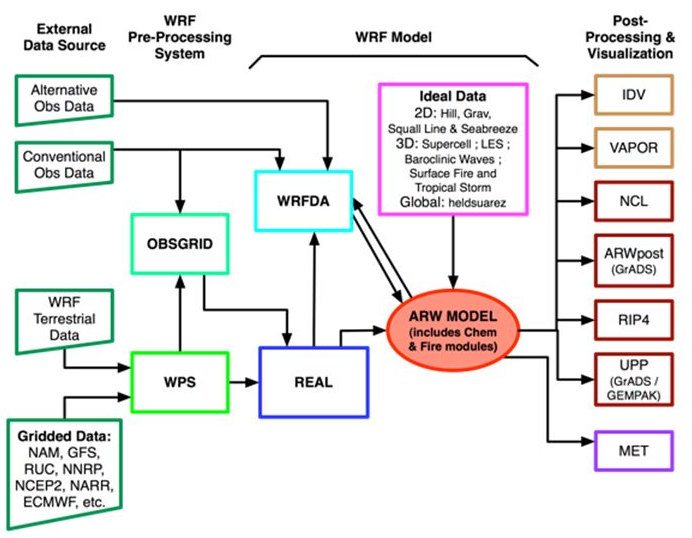
The WRF system is summarized in the following figure:

WRF flowchart

The ROMS and SWAN domain comprises the whole Adriatic Sea basin with 1 km horizontal grid resolution. The only open lateral boundary is located at the strait of Otranto (grid points located into the Ionian Sea have been masked out).

The ROMS vertical grid has 30 σ-layers and the bathymetry was obtained from the USGS Adriatic Sea Relief Model (15 arc sec) by bilinear interpolation over the model grid. The minimum depth is 8 meters and all the depths shallower than 8 have been replaced by this value.

57 riverine sources of fresh water have been incorporated into the model. The mass flow rate is provided on a daily basis as computed from climatological monthly averages coming from various datasets (as decribed in Verri et al., 2018) except for the Po river, whose flow rate is provided from daily observations transmitted in real time by the hydrometric station at Pontelagoscuro. The Po run-off is splitted into several grid points, according to the partitioning of the flow into the Delta, as described by Zasso and Settin (2012).

The lateral boundary conditions for temperature, salinity and velocity are taken from the Mediterranean Forecasting System (MFS) daily averages. The tidal signal is transmitted into the model through the lateral open boundary conditions on barotropic velocities according to Flather (1976) and to the free-surface following Chapman (1985).

ROMS is a free-surface, terrain-following numerical model that solves the three-dimensional Reynolds Averaged Navier-Stokes equations (RANS) using the hydrostatic and Boussinesq approximations. ROMS uses finite difference approximations on a horizontal curvilinear Arakawa C grid and on a vertical stretched terrain-following coordinate. Momentum and scalar advection and diffusive processes are solved using transport equations. An equation of state computes the density field that accounts for temperature, salinity and suspended sediment contributions.

ROMS provides a flexible structure that allows multiple choices for many of the model components, such as several options for advection schemes, turbulence models, lateral boundary conditions, bottom and surface boundary layer sub-models, air-sea fluxes, surface drifters, nutrient-phytoplankton-zooplankton-detritus models and an adjoint module to compute model inverses and data assimilation.

The hydrostatic primitive equations for momentum are solved using a split-explicit time stepping scheme which requires special treatement and coupling between barotropic (fast) and baroclinic (slow) modes. A finite number of barotropic time steps, within each baroclinic time step is carried out to evolve the free-surface and vertically integrated momentum equations. In order to avoid the errors associated with the aliasing of frequencies resolved by the barotropic steps, but unresolved by the baroclinic step, the barotropic fields are time averaged before they replace those values obtained with a longer baroclinic step.

The SWAN model shares the same computational grid as ROMS. To warm-up the model a hotstart file from the previous run is used. The lateral open boundary conditions are provided from the operational forecasting system SWAN-ITA (Cacciamani et al., 2012).

SWAN is a third generation spectral wave model specifically designed for shallow water that solves the spectral density evolution equation. SWAN simulates wind wave generation and propagation in coastal waters and includes the processes of refraction, diffraction, shoaling, wave-wave interactions and dissipation due to whitecapping, wave breaking and bottom friction.

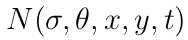
The wave model solves the action balance equation:

action balance equation

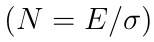
where action density spectrum is the action density spectrum, σ is the relative radiant frequency (as observed in a frame moving with the ocean current), θ is direction normal to wave crest, x and y are coordinate space and t is time. The action density is defined as the wave energy density E divided by the relative frequency relative frequency and is solved because the action density is conserved in the presence of currents. The group velocities in x and y directions cx and cy in the second and third terms represent the propagation of the action density in geographic space, the fourth term represents changes in relative frequency due to variations in depth and currents with a propagation speed cσ in frequency space and the fifth term allows depth and current-induced refraction with a speed cθ in directional space. The Sw term represents sources and sinks of wave energy density.
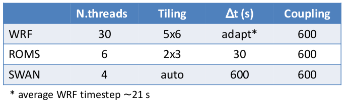
The three models run simultaneously on a High Performance machine with 2 Intel® Xeon® CPU E5-2680 v2 @ 2.80GHz processors in hyperthreading configuration for a total of 40 thread siblings. WRF is the component which requires the higher computational resources, hence it has been assigned 30 siblings, whereas ROMS has been assigned 6 and SWAN 2.

MCT setup

The time interval between coupling of models is 600 s.

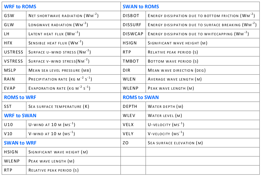
The table below summarizes the physical parameters exchanged between models by means of MCT:

MCT coupler parameters

The MCT coupler allows the transmission and transformation of various distributed data between component models using a parallel coupled approach. MCT is a program written in Fortran90 and works with the MPI communication protocol. It is compiled as a set of libraries, which are linked to the model executable.

At the initialization phase each model decomposes its own domain into sections (or segments) that are distributed to processors assigned for that component. Each grid section on each processors initializes into MCT and the coupler compiles a global map to determine the distribution of model segments. Each segment also initializes an attribute vector that contains the fields to be exchanged and establishes a router to provide an exchange pathway between model components.

During the run phase of the simulation the models will reach a predetermined syncronization point, fill the attribute vectors with data and use MCT send and receive commands to exchange fields.

REFERENCES

Booij, N., R.C. Ris, and L.H. Holthuijsen, 1999: A third-generation wave model for coastal regions: 1. Model description and validation. Journal of Geophysical Research: Oceans, 104, C4, 7649-7666. doi:10.1029/98JC02622

Cacciamani, C., M. Deserti, A. Valentini, S. Nanni, and T. Paccagnella, 2012: ARPA-SIMC Operational Oceanography for the Emilia-Romagna Support Centre and Centre of Competence of the National Civil Protection System. In: Operational Oceanography in Italy toward a suistainable management of the sea. I quaderni di Arpa, 201-209.

Chapman, D.C., 1985: Numerical Treatment of Cross-Shelf Open Boundaries in a Barotropic Coastal Ocean Model. Journal of Physical Oceanography, 15, 1060-1075. doi:10.1175/1520-0485(1985)015<1060:NTOCSO>2.0.CO;2

Flather, R.A., 1976: A tidal model of the northwest European continental shelf. Memoires de la Societe Royale de Sciences de Liege, 10, 141-164.

Haidvogel, D.B., H. Arango, W.P. Budgell, B.D. Cornuelle, E. Curchitser, E. Di Lorenzo, K. Fennel, W.R. Geyer, A.J. Hermann, L. Lanerolle, J. Levin, J.C. McWilliams, A.J. Miller, A.M. Moore, T.M. Powell, A.F. Shchepetkin, C.R. Sherwood, R.P. Signell, J.C. Warner, and J. Wilkin, 2008: Ocean forecasting in terrain-following coordinates: Formulation and skill assessment of the Regional Ocean Modeling System. Journal of Computational Physics, 227, 3595-3624. doi:10.1016/j.jcp.2007.06.016

Holthuijsen, L.H., 2007: Waves in Oceanic and Coastal Waters. Cambridge University Press, 404 pp. doi:10.1017/CBO9780511618536

Jacob, R., J. Larson, and E. Ong, 2005: M × N Communication and Parallel Interpolation in Community Climate System Model Version 3 Using the Model Coupling Toolkit. The International Journal of High Performance Computing Applications, 19, 293-307. doi:10.1177/1094342005056116

Larson, J., R. Jacob, and E. Ong, 2005: The Model Coupling Toolkit: A New Fortran90 Toolkit for Building Multiphysics Parallel Coupled Models. The International Journal of High Performance Computing Applications, 19, 277-292. doi:10.1177/1094342005056115

Maiello, I., R. Ferretti, S. Gentile, M. Montopoli, E. Picciotti, F.S. Marzano, and C. Faccani, 2014: Impact of radar data assimilation for the simulation of a heavy rainfall case in central Italy using WRF-3DVAR. Atmospheric Measurement Techniques, 7, 2919-2935. doi:10.5194/amt-7-2919-2014

Mazzarella, V., I. Maiello, V. Capozzi, G. Budillon, and R. Ferretti, 2017: Comparison between 3D-Var and 4D-Var data assimilation methods for the simulation of a heavy rainfall case in central Italy. Advances in Science & Research, 14, 271-278. doi:10.5194/asr-14-271-2017

Pinardi, N., I. Allen, E. Demirov, P. De Mey, G. Korres, A. Lascaratos, P.Y. Le Traon, C. Maillard, G. Manzella, and C. Tziavos, 2003: The Mediterranean ocean forecasting system: first phase of implementation (1998-2001). Annales Geophysicae, 21, 3-20. doi:10.5194/angeo-21-3-2003

Shchepetkin, A.F., and J.C. McWilliams, 2005: The regional oceanic modeling system (ROMS): a split-explicit, free-surface, topography-following-coordinate oceanic model. Ocean Modelling, 9, 347-404. doi:10.1016/j.ocemod.2004.08.002

Skamarock, W.C., J.B. Klemp, J.Dudhia, D.O.Gill, D.M.Barker, M.G. Duda, X.Y. Huang, W. Wang, and J.G. Powers, 2008: A Description of the Advanced Research WRF Version 3. NCAR Tech. Note NCAR/TN-475+STR, 113 pp. doi:10.5065/D68S4MVH

Tonani, M., N. Pinardi, S. Dobricic, I. Pujol, and C. Fratianni, 2008: A high-resolution free-surface model of the Mediterranean Sea. Ocean Science, 4, 1-14. doi:10.5194/os-4-1-2008

Verri, G., N. Pinardi, P. Oddo, S.A. Ciliberti and G. Coppini, 2018: River runoff influences on the Central Mediterranean overturning circulation. Climate Dynamics, 50, 1675-1703. doi:10.1007/s00382-017-3715-9

Warner, J.C., C.R. Sherwood, R.P. Signell, C.K. Harris, and H.G. Arango, 2008: Development of a three-dimensional, regional, coupled wave, current, and sediment-transport model. Computers & Geosciences, 34, 1284-1306. doi:10.1016/j.cageo.2008.02.012

Warner, J.C., B. Armstrong, R. He, and J.B. Zambon, 2010: Development of a Coupled Ocean-Atmosphere-Wave-Sediment Transport (COAWST) Modeling System. Ocean Modelling, 35, 230-244. doi:10.1016/j.ocemod.2010.07.010

Zasso, M., and T. Settin, 2012: Sulla ripartizione delle portate del Po tra i vari rami e le bocche a mare del delta: esperienze storiche e nuove indagini all'anno 2011. ARPAV Relazione n.02/12. 47 pp.